Why Everyone, Yes Everyone, Should Learn Statistics

Why Everyone, Yes Everyone, Should Learn Statistics

Simpson's Paradox
Simpson's Paradox: The correlation between two variables can change (even reverse!) when additional variables are considered

Simpson's Paradox
Simpson's Paradox: The correlation between two variables can change (even reverse!) when additional variables are considered
Example Code
ggplot(data = gapminder, aes(x = gdpPercap, y = lifeExp, color = continent, fill= continent))+ geom_point()+geom_smooth(method = "lm") + scale_x_log10()+ylab("Life Expectancy (Years)")+ xlab("Log GDP/Capita")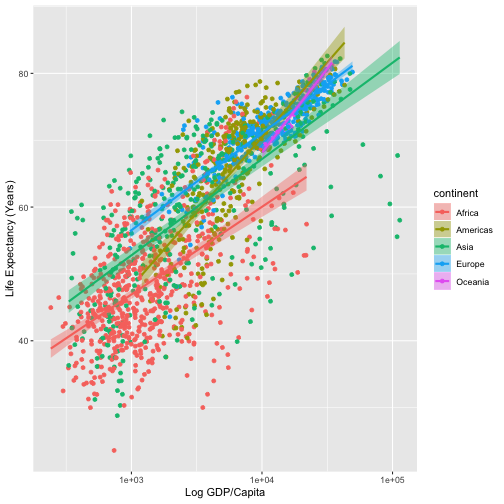
This Class Is
This Class Is
Example II
## ## Call:## lm(formula = hwy ~ displ, data = mpg)## ## Residuals:## Min 1Q Median 3Q Max ## -7.1039 -2.1646 -0.2242 2.0589 15.0105 ## ## Coefficients:## Estimate Std. Error t value Pr(>|t|) ## (Intercept) 35.6977 0.7204 49.55 <2e-16 ***## displ -3.5306 0.1945 -18.15 <2e-16 ***## ---## Signif. codes: 0 '***' 0.001 '**' 0.01 '*' 0.05 '.' 0.1 ' ' 1## ## Residual standard error: 3.836 on 232 degrees of freedom## Multiple R-squared: 0.5868, Adjusted R-squared: 0.585 ## F-statistic: 329.5 on 1 and 232 DF, p-value: < 2.2e-16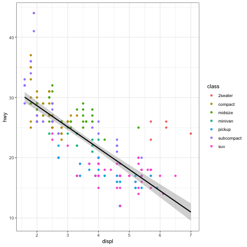
- Probability a student gets between a 65 and 85:
## [1] 0.6826895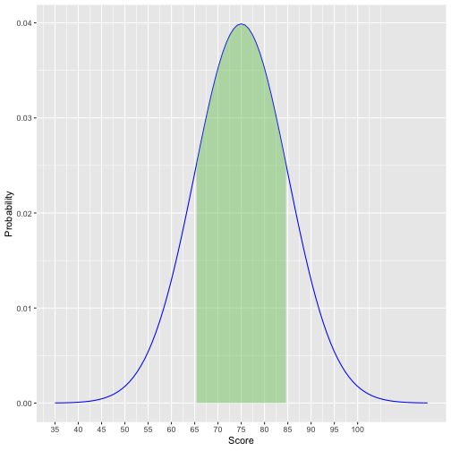
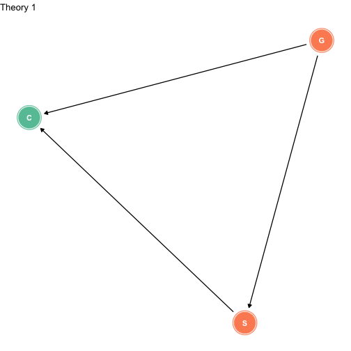
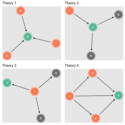
DAGs